This is an example of writing an R package using the Literate
Programming (LP) technique,
implemented through the knitr package and Makefile. It only shows you the
idea, and I do not mean you must use knitr, R Markdown, or Makefile. The
full source code of this rlp package is available on
Github. To build this package, you need to
install R packages knitr and rmarkdown. Windows users also need to
install Rtools, which includes
the utility make. Linux and macOS users should have make ready by default.
Literate Programming
Interestingly, the most popular application of the LP paradigm seems to be
documenting software (using a special form of comments) for users instead of
“programming” for authors. In other words, we use LP to document the usage of
software, instead of documenting the source code. See
Doxygen,
Javadoc, and
roxygen2 for examples. There
exists one exception, though, in the LaTeX world1. Some LaTeX package authors
write both LaTeX code and documentation in a single document, and weave it into
a PDF document that contains both the source code and documentation. I’m not a
LaTeX expert, and it is probably well-known that I have big headache when
looking at a full screen of backslashes, from \documentclass{},
\begin{document}, \alpha, \beta, \texttt{}, …, and all the way to
\end{document}.
I do not find LP for LaTeX appealing, but that does not mean LP itself is not an appealing idea. On the contrary, I believe it can be very interesting and useful when it is applied to your own favorite language, e.g., R for me. In my opinion, LP has at least two advantages:
- You can write much more extensive and richer documentation than you normally could do with comments. In general, comments in code are (or should be) brief and limited to plain text. Normally you will not write five paragraphs of comments to explain a few lines of code, and you cannot write readable2 math expressions or embed a video in comments.
- You can label code chunks and reference/reuse them using the labels, which allows you to compose your program flexibly using different pieces of code chunks. For example, you can define and explain a code chunk later in the document, but insert it in a previous code chunk using its label. This feature has been emphasized by Knuth, but I do not see it is widely adopted for some reason. Perhaps most people are more comfortable with designing a big program by smaller units like functions instead of code chunks, which is actually a good idea.
Personally I find the first advantage more convincing, although it seems some LP folks just love the second one. For R package development, I guess it will be inconvenient for unit testing if we use the LP idea instead of writing smaller functions, because testing functions is straightforward, but testing code chunks is not. Anyway, I will show both features of LP mentioned above in this document.
Setup
First, I set a few knitr chunk options:
knitr::opts_chunk$set(eval = FALSE, tidy = FALSE)
I set eval = FALSE because this document mostly serves as the documentation of
our R source code, and I do not really need to run the code chunks here. The
code will be generated to the R/ directory, then built by R CMD build into
an R package. If you do want to execute a code chunk, you can use the chunk
option eval = TRUE on that code chunk. Another important reason that you may
not want to evaluate some code chunks is that they may not be complete, for
example, when you insert documentation in the middle of a function to explain a
few lines of the function body.
In this document, you will see the chunk option purl = FALSE occasionally, and
that means I want to exclude these code chunks when extracting the R code, but I
do want to include them when compiling this document to HTML.
R Code Chunks
Now I write some example R code chunks using the R Markdown syntax. Here I
define a boring function add_one() with an argument x, and it simply does
x + 1:
#' A cool function
#'
#' Well, not really cool. Just add 1 to x.
#' @param x a numeric vector
#' @export
#' @examples
#' add_one(1)
#' add_one(1:10)
add_one = function(x) {
  x + 1
}
Besides the R source code, I also wrote the R documentation using the
roxygen2 syntax. This R code chunk will be extracted and placed under the
R/ directory later. The critical step is how to extract the code chunk. After
this step, you will be in a familiar world of roxygen2::roxygenize(), or
devtools::build(), or R CMD build, or whatever package building process you
like.
From Rmd to R
I put this Rmd file under the vignettes/ directory, and you do not have to use
this directory. I’m using it because I will get a nice by-product after
R CMD build, which is the package vignette. I used rmarkdown to generate
an HTML vignette, which is visually pleasant to read in my eyes.
To extract the code chunks from the Rmd documents, I used a Makefile under the
root directory of this package3:
purl=Rscript -e "knitr::purl('$(1)', '$(2)', quiet=TRUE, documentation=0)"

rfiles:=$(patsubst vignettes/LP-%.Rmd,R/%-GEN.R,$(wildcard vignettes/LP-*.Rmd))

all: $(rfiles)

R/%-GEN.R: vignettes/LP-%.Rmd
	$(call purl,$^,$@)
I defined a function purl in the Makefile, which calls the R function
knitr::purl() to extract code chunks from Rmd to R. To make sure I do not purl
arbitrary Rmd documents, I added a prefix LP- to the Rmd filenames, and only
these files will be processed. Similarly, to make sure make does not use
arbitrary R files as targets, I added a suffix -GEN (stands for “generated”)
to the R filenames. To put it short, an Rmd file vignettes/LP-foo.Rmd will
generate R/foo-GEN.R. The variable rfiles stores all the potential R scripts
to be generated. If you are familiar with make, you will immediately see its
advantage here: foo-GEN.R will be re-generated only if LP-foo.Rmd has been
updated.
You may have realized that this leads to two copies of R code: one copy in Rmd,
and one in R. Therefore you need to remind your collaborators (if you have any)
that they must not edit the R code under R/ that is generated from Rmd, but
should edit the Rmd source documents instead.4
One Button to Rule Them All
Now we have three things to do to fully build this package:
- Run
maketo generate R source code toR/; - Run roxygen2 to generate R documentation to
man/,NAMESPACE, and other stuff; - Run
R CMD buildto build the package as well as the vignettes.
You certainly do not want to type these commands repeatedly. Unfortunately, due to the fact that this is not the standard process of building an R package, there is not a natural solution to combine the three steps into one. For power users, this is certainly not true – you can always write a shell script to do everything. But some users just do not know how to open a terminal to type commands, and you should not blame them – not all people do programming for a living, and a command window is not the only or ultimate solution of all problems.
So let’s start hacking and find a button to click. I have been secretly hacking
the Build & Reload button in my RStudio IDE for a long time. If you open this
rlp package in RStudio, and go to Tools -> Project Options -> Build Tools,
you will see a weird configuration:
-v && Rscript -e "Rd2roxygen::rab(install=T,before=system('make'))"
At this moment, I’m not going to explain what it means since it is just a dirty hack, and please do not ask me, either. Let’s wait for the RStudio IDE to give us more freedom to customize the package build options in the future. If you are interested in the idea of LP for R packages, just copy my configuration, but bear in mind that it may stop working at some point. I will update this document when that happens.
Note Rd2roxygen::rab() is my own way of building R packages, and you certainly
do not have to follow it. For example, if you are more comfortable with
devtools, you can do5:
-v && make -C rlp && Rscript -e "devtools::install('rlp')"
Call Functions in This Package
You can certainly load the package and call the functions in this document,
because the package vignettes are compiled after the package is temporarily
installed6. For example, I call add_one() defined above:
library(rlp)
add_one(1)
## [1] 2
add_one(1:10)
## [1] 2 3 4 5 6 7 8 9 10 11
Running live examples and generating output like this may help you explain what your functions actually do, so readers can understand your source code better, otherwise they can only reason about the code in their mind.
A Less Naive Example
Life is certainly not always as simple as add_one(). In this section, I give a
slightly more advanced example to show how LP can be useful and relevant to
developing R packages. Let’s consider the maximum likelihood estimation (MLE)
for the parameters of the Gamma distribution \(\Gamma(y; \alpha, \beta)\).
I will use the function optim() to optimize the log-likelihood function.
First, I define an R function with arguments data and start:
#' MLE for the Gamma distribution
#'
#' Estimate the parameters (alpha and beta) of the Gamma distribution
#' using maximum likelihood.
#' @param data the data vector assumed to be generated from the Gamma
#'   distribution
#' @param start the initial values for the parameters of the Gamma
#' distribution (passed to \code{\link{optim}()})
#' @param vcov whether to return an approximate variance-covariance
#' matrix of the parameter vector
#' @return A list with elements \code{estimate} (parameter estimates
#'   for alpha and beta) and, if \code{vcov = TRUE}, \code{vcov} (the
#'   variance-covariance matrix of the parameter vector).
#' @export
mle_gamma = function(data, start = c(1, 1), vcov = FALSE) {
The Gamma distribution has two commonly used parameterizations (shape-rate or shape-scale), and I will use the following probability density function (shape-rate):
$$f(x|\alpha,\beta)=\frac{\beta^{\alpha}}{\Gamma(\alpha)}x^{\alpha-1}\exp(-\beta x);\quad x>0$$
The log-density function is:
$$\log f=\alpha\log\beta-\log\Gamma(\alpha)+(\alpha-1)\log x-\beta x$$
The log-likelihood function given the data vector
\(\mathbf{x}=[x_1,x_2,\ldots,x_n]\) will be:
$$L(\alpha,\beta|\mathbf{x})=n(\alpha\log(\beta)-\log(\Gamma(\alpha)))+(\alpha-1)\sum_{i=1}^{n}\log(x_{i})-\beta\sum_{i=1}^{n}x_{i}$$
And I define it in R as loglike(), where param is the parameter vector
\([\alpha, \beta]\), and x is the data vector:
  loglike = function(param, x) {
    a = param[1]  # alpha (the shape parameter)
    b = param[2]  # beta (the rate parameter)
    n = length(x)
    n * (a * log(b) - lgamma(a)) + (a - 1) * sum(log(x)) - b * sum(x)
  }
It is worth noting that in practice we will rarely translate the math equation
to R code like that for the Gamma distribution, since R has the dgamma()
function that is much more efficient than the raw log-density function I used
above. You would use
sum(dgamma(x, shape = param[1], rate = param[2], log = TRUE)) instead. Anyway,
I took the silly way just for demonstrating the LP idea instead of how to write
efficient statistical computing code.
Next I optimize the log-likelihood function by passing the initial guesses and the data vector to it:
opt = optim(start, loglike, x = data, hessian = vcov, control = list(fnscale = -1))
You need to be cautious that optim() minimizes the objective function by
default, and that is why I used control = list(fnscale = -1). Then I’m
minimizing -loglike, and essentially maximizing loglike. I need to make sure
the optimization has reached convergence:
  if (opt$convergence != 0) stop('optim() failed to converge')
  res = list(estimate = opt$par)
Finally, I give an estimate of the variance-covariance matrix
\(Var([\hat{\alpha},\hat{\beta}]')\) if vcov = TRUE:
if (vcov) res$vcov = solve(-opt$hessian)
The estimate is the inverse of the negative Hessian matrix, because
\(Var(\hat{\theta})=I^{-1}(\theta)\) for the maximum likelihood estimator
\(\hat{\theta}\), where \(I(\theta)\) is the Information matrix, and we know
\(I(\theta) = -E(H(\theta))\). In theory, \(I(\theta)\) is unknown, and I just use
the observed information matrix, i.e., the negative Hessian matrix returned from
optim(). Note the inverse matrix is computed via solve().
  res
}
The object res is returned, and we can use it to compute the confidence
intervals of the parameters since MLE is asymptotically Normal. Now let’s try
the function:
set.seed(1228)
d = rgamma(100, shape = 5, rate = 2)  # simulate some data from Gamma(5, 2)
r = mle_gamma(d, vcov = TRUE)
str(r)
## List of 2
##  $ estimate: num [1:2] 5.3 2.06
##  $ vcov    : num [1:2, 1:2] 0.529 0.206 0.206 0.088
The estimates are not too bad, compared to their true values. I can also give a
95% confidence interval for the parameter \(\alpha\), of which the estimate is
asymptotically Normal:
a = r$estimate[1]  # estimate of alpha
s = sqrt(r$vcov[1, 1])  # standard error of the estimate of alpha
z = qnorm(1 - 0.05/2)  # 97.5% Normal quantile
c(a - z * s, a + z * s)  # a 95% CI
## [1] 3.876 6.727
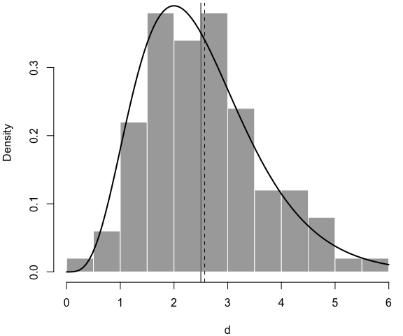
Below is a histogram of the simulated data, with the true density curve, the true mean (solid vertical line), and the estimated mean (dashed line):7
par(mar = c(4, 4, .2, .1))
hist(d, main = '', col = 'darkgray', border = 'white', freq = FALSE)
curve(dgamma(x, shape = 5, rate = 2), 0, 6, add = TRUE, lwd = 2)
abline(v = c(5/2, r$estimate[1]/r$estimate[2]), lty = c(1, 2))
Now you see I can thoroughly explain an R function using LP. I’m not saying this is what you should do for all R functions, but sometimes there are cases in which you want something beyond code comments, such as math equations and graphics.
Apparently LP is more for those who want to understand your source code
(including your future self!) than for end-users of your package. For most
users, they probably just want to read the help page of the function, in which
case they just type the question mark in R, e.g., ?mle_gamma.
Chunk References
I mentioned before that we could label code chunks and reference them to compose a bigger code chunk. Now I show a simple example of simulating from a bivariate Normal distribution. A bit background:
$$\left[\begin{array}{c} X\\ Y \end{array}\right]\sim\mathcal{N}\left(\left[\begin{array}{c} \mu_{X}\\ \mu_{Y} \end{array}\right],\left[\begin{array}{cc} \sigma_{X}^{2} & \rho\sigma_{X}\sigma_{Y}\\ \rho\sigma_{X}\sigma_{Y} & \sigma_{Y}^{2} \end{array}\right]\right)$$
One way to simulate from the bivariate Normal distribution is to first simulate
from the marginal distribution \(f(x)\), then simulate from \(f(y|x)\). Below is the
final simulation function:
#' Sample from a bivariate Normal distribution
#'
#' Simulate x from the marginal f(x), then y from f(y|x), and
#' the pair (x, y) has the desired joint distribution.
#' @param n the desired sample size
#' @param m1,m2 the means of X and Y, respectively
#' @param s1,s2 the standard deviations of X and Y, respectively
#' @param rho the correlation coefficient between X and Y
#' @return A numeric matrix of two columns X and Y.
#' @export
rbinormal = function(n, m1 = 0, m2 = 0, s1 = 1, s2 = 1, rho = 0) {
  # warning: this is not an efficient implementation; you should use
  # vectorization in practice
  res = replicate(n, {
    x = rnorm(1, m1, s1)  # simulate from the marginal f(x)
    m2cond = m2 + s2/s1 * rho * (x - m1)  # conditional mean of Y
    s2cond = sqrt(1 - rho^2) * s2  # conditional sd of Y
    y = rnorm(1, m2cond, s2cond)  # simulate from the conditional f(y|x)
    c(x, y)
  })
  res = t(res)  # transpose the 2xn matrix to nx2
  colnames(res) = c('X', 'Y')
  res
}
If you are reading the source R Markdown
document, you
will see <<simulate_x>> and <<simulate_y>> instead of the real R code. The
token <<>> denotes the code chunks defined below with the chunk labels
simulate_x and simulate_y, respectively:
x = rnorm(1, m1, s1) # simulate from the marginal f(x)
The marginal distribution of \(X\) is \(\mathcal{N}(\mu_X, \sigma^2_X)\), and we
know the conditional distribution of \(Y|X\) is:
$$Y|X=x \sim \mathcal{N}\left(\mu_{Y}+\frac{\sigma_{Y}}{\sigma_{X}}\rho(x-\mu_{X}),\,(1-\rho^{2})\sigma_{Y}^{2}\right)$$
m2cond = m2 + s2/s1 * rho * (x - m1)  # conditional mean of Y
s2cond = sqrt(1 - rho^2) * s2  # conditional sd of Y
y = rnorm(1, m2cond, s2cond)  # simulate from the conditional f(y|x)
I just reused these code chunks in the function body of rbinormal(), instead
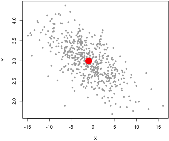
of cutting and pasting the code there. As usual, I can test my function by
examples:
set.seed(1229)
z = rbinormal(500, m1 = -1, s1 = 5, m2 = 3, s2 = .5, rho = -.7)
par(mar = c(4, 4, .2, .1))
plot(z, pch = 20, col = 'darkgray')
# the center of the bivariate dist
points(-1, 3, pch = 19, col = 'red', cex = 3)
In this example, I factored out the code from the main function as two separate code chunks, and explained each later, instead of inserting the explanations in the middle of the function body. Again, the simulation code in this example is computationally inefficient, and it is only for demo purposes8.
Conclusions
This document has demonstrated that LP can be useful for package authors to explain their code in fine detail, which may not be easy to achieve by only using comments in code. Not everyone needs or wants to understand your source code, but clear explanations of your code will benefit both your future self, and more importantly, attract potential collaborators and contributors, hence increase the bus factor of your software packages, in this era of “social coding”.
-
This is not entirely surprising, considering Knuth’s original implementation of LP using TeX and Pascal. ↩︎
-
By “readable”, I mean no backslashes. Raw LaTeX math code does not count. At least it is not readable to me. I can never figure out where the brackets start and end by reading raw LaTeX code, for example, when there are more than three pairs of brackets. ↩︎
-
If you read the R Markdown source of this document, you will see I did not copy the Makefile here, but used the
catengine to write the Makefile dynamically to the output. ↩︎ -
Or set the R scripts to be read-only, e.g., use
Sys.chmod(mode = '0444')in R. ↩︎ -
Remember to replace
rlpwith your package name. ↩︎ -
If you use devtools, please note it does not build vignettes by default, so you have to call
devtools::install(..., build_vignettes = TRUE)↩︎ -
The mean of the Gamma distribution is
\(\alpha/\beta\). ↩︎ -
It is straightforward to make it much more efficient by vectorization, i.e., instead of using
replicate(), which is basically a loop to generate one random number at a time, you can just generate allnrandom numbers in one step:x = rnorm(n, m1, s1), andy = rnorm(n, m2cond, s2cond). ↩︎