晚上陈淼同学问我一个关于二元函数单调性的问题,最近我也没有准备复习考研,所以数学分析也没看,脑子里没有一点数学思维了。拿起题目一看,有些傻眼,不知该咋个整。函数是这样的:
$$f(d,u)={1/(d-u)-(\log(d/u))*u/(d-u)^2},\quad d\in(0.5,1),,u\in(0,0.5)$$
目的是想知道f什么时候取最小值,我在S-Plus中实现的步骤如下(注意,我的S-Plus是自己设置过的,这里的":)“就是一般见到的”>“表示另一段完整的程序语句开始,而”^^“就是一般的”+“表示续行,我只不过觉得S-Plus默认的不好玩,所以这样设置了一下——题外话):
:) d_seq(0.51,1,0.01)
:) u_seq(0,0.49,0.01)
:) f_function(d,u)
^^ {1/(d-u)-(log(d/u))*u/(d-u)^2}
:) d_seq(0.51,1,0.01)
:) u_seq(0,0.49,0.01)
:) persp(d,u,outer(d,u,FUN="f"),"d","u","f")
注意看我对d和u的设置,把定义域稍微缩小了一点点,原因是d和u的定义域都不包括边界,另一个目的是因为后面用到outer函数时可能会涉及到d-u可能等于0的问题(不可作分母),所以我去掉了边界0.5。上面的f是一个自定义函数没什么好说的,关键在于两个函数outer和persp,我长话短说吧,具体说明自己看文章最后的英文:)outer的作用是把两个向量的元素依次遍历使用FUN函数作用得到一个新的数组(或者矩阵),因此,其元素个数就是两个向量的长度(元素个数)之积。注意理解什么叫遍历!其实就类似于一个二重循环。persp的作用在于作出三维图,三个参数依次使用x,y,z坐标,要注意的是z坐标比较特殊,z[i,j]是与x[i]和y[j]对应的;现在再回过头去理解一下outer函数的意义所在吧。
不知道是否说清楚了,输出图形如下:
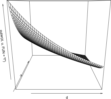
很容易就知道,当d和u分别尽量大时,f值会尽量小,同时单调性也显而易见。至于严格证明,我懒得花时间证了,思路就是固定一个变量,然后用作差法看单调性,应该没问题的(高中数学问题)。
附:下面是对outer函数和persp函数的详细说明——
**Outer**

**DESCRIPTION**


Performs an outer product operation given two arrays (or vectors) and, optionally, a function.


**USAGE**


outer(X, Y, FUN="*", ...)


X %o% Y #operator form


**REQUIRED ARGUMENTS**


X,Y   first and second arguments to the function FUN. Missing values (NAs) are allowed if FUN accepts them.


**OPTIONAL ARGUMENTS**


FUN   an S-PLUS function that takes at least two vectors as arguments and returns a single value. This may also be a character string giving the name of such a function.
   ...   other arguments to FUN, if needed.  The names of the arguments, if any, should be those meaningful to FUN.


**VALUE**


array, whose dimension vector is the concatenation of the dimension vectors of X and Y, and such that FUN(X[i,j,k,...], Y[a,b,c,...]) is the value of the [i,j,k,...,a,b,c,...] element. (Vectors are considered to be one-dimensional arrays.)


**DETAILS**


outer forms two arrays corresponding to the data in X and Y, each of which has a dim attribute formed by concatenating the dim attributes of X and Y. It then calls FUN just once with these two arrays as arguments. Therefore, FUN should be a function that operates elementwise on vectors or arrays and expects (at least) two arguments.


**SEE ALSO**


crossprod, Matrix-product.


**EXAMPLES**


z <- x %o% y   # The outer product array


# dim(z) == c(dim(as.array(x)), dim(as.array(y)))


# simulate a two-way table


outer(c(3.1, 4.5, 2.8, 5.2), c(2.7, 3.1, 2.8),"+") + matrix(rnorm(12), nrow=4)


z <- outer(months, years, paste) # All month, year combinations pasted.


**Persp**


**DESCRIPTION**


Creates a perspective plot given a matrix that represents heights on an evenly spaced grid. Axes and/or a box may be placed on the plot.


**USAGE**


persp(x, y, z, xlab = "X", ylab = "Y", zlab = "Z", axes = T,
      box = T, eye = <<SEE below="" />>, zlim = <<SEE below="" />>, ar = 1)


**REQUIRED ARGUMENTS**


x   vector containing x coordinates of the grid over  which  z is evaluated. The values should be in sorted order; missing values are not accepted.
y   vector of grid y coordinates. The values should be in sorted order; missing values are not accepted.
z   matrix of size length(x) by length(y) giving  the  surface height  at grid points, i.e., z[i,j] is evaluated at x[i], y[j].  The rows of z are indexed by x, and the columns  by y.  Missing values (NAs) are allowed, but should generally not occur in the convex hull of the non-missing values.


The first argument may be a list with components x, y, and z. In particular, the result of interp is suitable.


If the first argument is a matrix, it is assumed to be the z matrix and vectors x and y are generated (x is 1:nrow(z), y is 1:ncol(z)).   The result of
predict together with expand.grid is suitable as an argument to persp.


**OPTIONAL ARGUMENTS**


xlab   character label for the x axis.
ylab   character label for the y axis.
zlab   character label for the z axis.
eye   vector giving the x,y,z coordinates for the viewpoint. The default is c(-6, -8, 5) times the range of the x, y, and z values.
axes   logical flag: should axes be drawn around the surface?
box   logical flag: should a box be drawn around the surface?


zlim   vector of the desired minimum and maximum z axis values.  The default is the range(z, na.rm=T).  This range will be expanded to round numbers.  The values in the input matrix z will be truncated to the z axis limits.
ar   aspect ratio for plotting the x,y grid, i.e., (xmax-xmin)/(ymax-ymin).


Graphical parameters may also be supplied as arguments to this function (see par).


**NOTE**


persp assumes that the grid vectors x and y are increasing and evenly spaced.  If this is not true, suppress the axes with axes=F or use par commands to customize the axes.


**VALUE**


invisible list containing information about what was plotted.


rotation   integer flag between 1 and 4 describing the point of view based on which corner of the xy plane appears closest to the viewer.
proj   2 by 2 by 2 array describing the projection of vectors that span the data.
rangex   vector giving the min and max values for x.
rangey   vector giving the min and max values for y.
rangez   vector giving the min and max values for z.


**SIDE EFFECTS**


a perspective plot is created on the current graphics device.


**DETAILS**


Use persp.setup to change the color, line width and line type of the perspective lines.  Use the perspp function to add information to a perspective plot.


**BUGS**


For some plots (including the case where mfrow or mfcol is bigger than c(2,2)) parts of the axes are cut off.  You can solve this problem either by putting up fewer figures on the page, changing the perspective angle with the eye argument, or by expanding the margin in which the cut off occurs.


Lines with an endpoint outside the plot may not be drawn.


**SEE ALSO**


contour, expand.grid, image, interp, outer, par, persp.setup, perspp, predict.


**EXAMPLES**


#Example 1, a polynomial


poly1 <-function(x, y){x^2 + x * y + y^2}
y <- x <- seq(-25, 25, length = 50)
persp(x,y, outer(x,y, FUN =  poly1))


#Example 2, data at geographic points
i <- interp(ozone.xy$x,ozone.xy$y,ozone.median)
persp(i, xlab = "Longitude", ylab = "Latitude", zlab = "Ozone")
title(main = "Median Ozone Concentrations in the North East")


#Example 3, first argument is a matrix
persp(switzerland)


#Example 4, a smooth surface
int.ak <- interp(akima.x, akima.y, akima.z)
r.ak <- sapply(int.ak, function(x) diff(range(x,na.rm = T)))


par(mfrow = c(2,2), oma = c(0,0,5,0))
persp(int.ak)
persp(int.ak, eye = c(6,-8,5)*r.ak)
persp(int.ak, eye = c(6,8,5)*r.ak)
persp(int.ak, eye = c(-6,8,5)*r.ak)
mtext(outer = T, side = 3, line = 2, "WAVEFORM DISTORTION", cex = 1.5)


par(mfrow = c(1,1))
persp(int.ak, eye = c(6,8,5)*r.ak)
title(main = "WAVEFORM DISTORTION")