For beginners, it is probably a good idea to start with some minimal examples; here I provide a few examples for Rnw, LaTeX, Markdown and HTML, respectively.
How is a report generated from R code
Regardless of which format you use, the basic idea is the same: knitr extracts R code in the input document, evaluates it and writes the results to the output document. There are two types of R code: chunks (code as separate paragraphs) and inline R code. For example, here we show a code chunk (using traditional Sweave syntax):
Example text outside R code here; we know the value of
pi is \Sexpr{pi}.
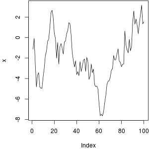
<<my-label, eval=TRUE, dev='png'>>=
set.seed(1213)  # for reproducibility
x = cumsum(rnorm(100))
mean(x)  # mean of x
plot(x, type = 'l')  # Brownian motion
@
Other text outside R code here.
After weaving this chunk, we get the output as below. Compare them and you will realize the inline code \Sexpr{pi} is replaced by the value of pi, and the code chunk is also evaluated – numerical results are printed and plots are inserted in the output as well.
Example text outside R code here; we know the value of
pi is 3.1415926.
set.seed(1213)  # for reproducibility
x = cumsum(rnorm(100))
mean(x)  # mean of x
## [1] -1.939758
plot(x, type = 'l')  # Brownian motion
Other text outside R code here.
Now hopefully you have got an idea of how automatic report generation works. There are many options of which we can make use to tune the results, for example, we can use echo=FALSE to hide the R souce code (usually you do not want R code to appear in a final report, unless you are writing a tutorial on R), or results='hide' to hide the printed results (e.g. you will not see ## [1] -1.939758 above if you use this option), or control the format, size and alignment of plots. Beside local chunk options which you write between << and >>=, you can also set options globally like:
knitr::opts_chunk$set(
  echo = FALSE, fig.path = 'myproject/plot-', cache = TRUE
)
Once options are set globally, all the following chunks will be affected by these options, so if you use an option frequently in many chunks, you may want to set it globally.
The advantage of using knitr is obvious: you only maintain the source code, and whenever you want a report, you just knit the source code, and everything will be generated automatically (tables, plots and numbers in lines). There is no need to manually copy and paste anything. Next time if you data source is changed, you simply run the process again, and all results can be updated. Let computers do the tedious job, because this is what they are good at. Humans should focus on other jobs like the statistical analysis and organization of the report.
Examples
Two main differences among different file formats are: they use different syntax to wrap up R code in the input document (see patterns), and the results returned from R are marked up according to the syntax of the output document (see hooks). For instance, Rnw uses << and >>=, and HTML uses <--!begin.rcode and end.rcode--> for the input; plots will be put in \includegraphics{...} for LaTeX output, and in <img src=...> for HTML output.
- Rnw
- Rnw source: knitr-minimal.Rnw
- PDF output: knitr-minimal.pdf
- a more minimal 002-minimal.Rnw (recommended for absolute beginners)
- Markdown
- example 1: 001-minimal.Rmd
- output: 001-minimal.md (GitHub does the job of parsing the md file to HTML)
- example 2: knitr-minimal.Rmd
- output: knitr-minimal.md
- HTML
- html source: knitr-minimal.Rhtml
- output: knitr-minimal.html
- LaTeX
- tex source: 005-latex.Rtex
- reStructuredText
- source: knitr-minimal.Rrst
- output: knitr-minimal.rst
You can run knit() to knit the input file, e.g.,
library(knitr)
knit('knitr-minimal.Rnw')
knit('knitr-minimal.Rhtml')
knit('knitr-minimal.Rmd')
Note for the HTML demo, you need to install the rgl package to get the snapshot in the output.
Some comments
One consideration in defining the default syntax for these files is that we should try not to break the syntax of other software systems, e.g. for LaTeX and HTML, the chunk options are written in comments, so the original document is still a valid TeX or HTML document. Unfortunately the original author(s) of literate programming did not seem to care about this issue at all, and invented the <<>>= + @ syntax; then Sweave added more pseudo-LaTeX commands like \SweaveOpts and \Sexpr; we cannot do much about them since they have been used for many years, and we are likely to be in bigger troubles if we break these rules. The LaTeX example above only serves as an example of how I would have defined the syntax, and you may not really want to follow it.
As a final side note, the extension Rnw is a combination of R + nw where nw stands for Noweb (= No + web), and WEB was coined by Donald Knuth to denote the idea of weaving documents. Today probably everybody will think of WWW when seeing the word web.