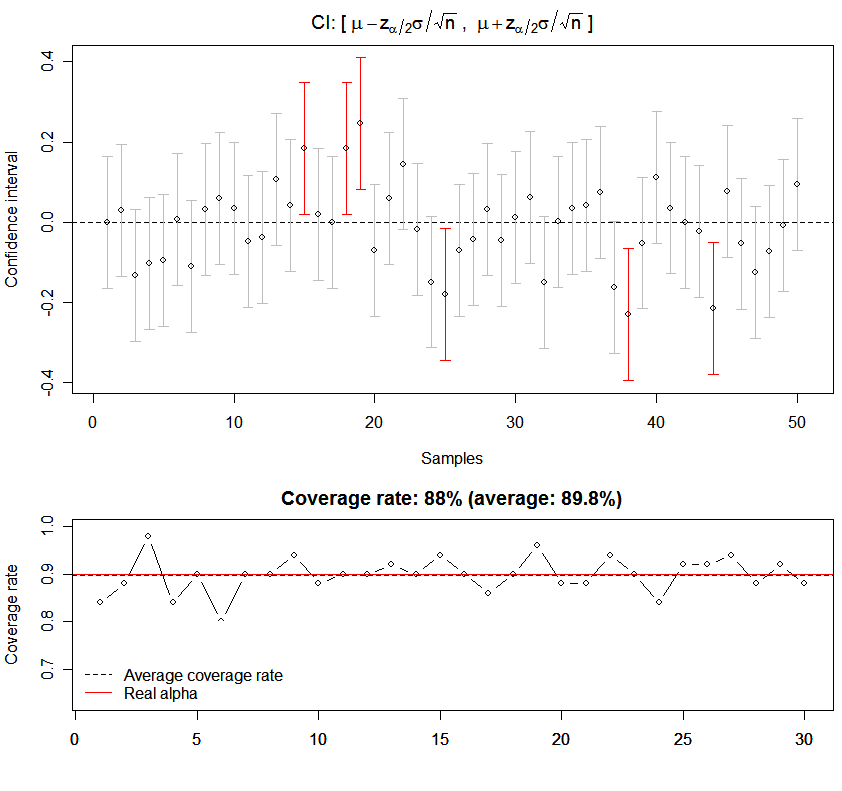
Demonstration of Confidence Intervals Using R (Animated)

[notice type=notice]NOTE: There's a typo in the graph! The $latex \mu$ should be replaced with the sample mean $latex \bar{x}$! And the code is available in the R package animation; see library(animation); ?conf.int

Yihui @ Dec 24, 2007

[/notice]

Recently I've been thinking about attending the conference of IASC2008, and my vague idea is to use animations in statistical education, especially in the demonstration of some algorithms containing iterations or loops. Perhaps the main difficulty just lies in an integrated theory -- currently I'm still not clear about the literature in this area (if anyone knows, please do drop me a line).

The other day when I was browsing the R documentation pages, I noticed that the amount of materials in those pages is increasing at a high speed. Among them I also saw some excellent web sites build by students (e.g. from Taiwan), which has triggered my own idea on building an independent website introducing animated pictures in statistics.

So... Let's come back to the topic. In fact this is a demonstration I made several weeks ago, and today I modified it a little bit in order that the coverage rate can be better shown. The idea behind this simulation is simple: draw samples (random numbers) from the population which follows N(0, 1), and calculate confidence intervals (CI) based on these samples respectively. I believe everybody surely knows the formula in the main title of the figure below (suppose sigma is known, then compute the CI for the unknown mu). Here is an "animated" PDF file:

[notice type=download]Downdload the file here[/notice]

R code for the demo:

[notice type=download]Downdload the file here[/notice]

###### arguments ######
# n: the number of samples used in the demo
# alpha: 1 - level of significance
# rn: sample size in each sample (different with n!)
# time: time interval between the drawing of CIs
# times: how many times should we compute the coverage rate
# (i.e. repeat the demo several times to check the coverage rate)
##### background ######
# X~N(mu, 1), we want to know the CI for mu
f = function(n = 100, alpha = 0.95, rn = 50, time = 0.1,
   times = 10) {
   par(mar = c(4.5, 4, 2.5, 0.5))
   layout(matrix(1:2, 2), heights = c(0.6, 0.4))
   ci = NULL
   for (j in 1:times) {
       d = replicate(n, rnorm(rn))
       m = colMeans(d)
       z = qnorm(1 - (1 - alpha)/2)
       y0 = m - z * 1/sqrt(rn)
       y1 = m + z * 1/sqrt(rn)
       plot(1, xlim = c(0.5, n + 0.5), ylim = c(min(y0), max(y1)),
           type = "n", xlab = "Samples", ylab = "Confidence interval",
           main = expression("CI: [" ~ mu - z[alpha/2] * sigma/sqrt(n) ~
               ", " ~ mu + z[alpha/2] * sigma/sqrt(n) ~ "]"))
       abline(h = 0, lty = 2)
       for (i in 1:n) {
           arrows(i, y0[i], i, y1[i], length = 0.05, angle = 90,
               code = 3, col = ifelse(0 > y0[i] & 0 < y1[i],
                 "gray", "red"))
           points(i, m[i])
           Sys.sleep(time)
       }
       ci = c(ci, mean(y0 < 0 & y1 > 0))
       plot(ci, xlim = c(1, times), ylim = c(0.7 * alpha, 1),
           xlab = "", ylab = "Coverage rate", type = "b", main = paste(
           "Coverage rate: ",
               ci[j] * 100, "%", " (average: ", round(mean(ci) *
                 100, 2), "%)", sep = ""))
       abline(h = mean(ci), lty = 2)
       abline(h = alpha, col = "red")
       legend("bottomleft", c("Average coverage rate", "Real alpha"),
           lty = c(2, 1), col = c("black", "red"), bty = "n")
       Sys.sleep(8)
   }
}

f(50, 0.9, 100, 0.1, 30)
# one demonstration