This demo was written by me about three months ago when I was illustrating the algorithm of Gradient Descent in the class of “Data Mining & Machine Learning”. I like to combine iterations (or loopings) with animated pictures, because it’s simple and heuristic, and of course, it’s easy in R: just use Sys.sleep() to control the time of steps of your demonstration and some low-level graphics functions such as lines(), points(), rect(), polygon() and segments(), etc to illustrate the process of your algorithm. To understand the figure below, you need to be clear about what’s contour plot.
Below is the code for the above example, and it has been included in the animation package as the grad.desc() function:
op = par(
pty = "s", mar = c(2, 1, 2, 0), cex.axis = 0.75, cex.main = 0.85
)
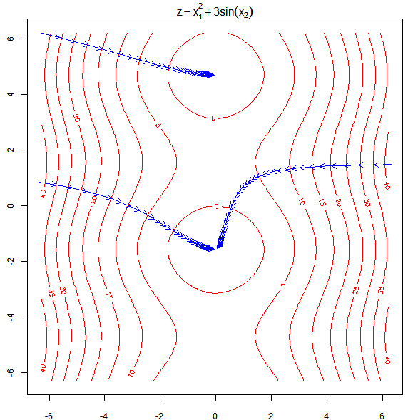
x2 = x1 = seq(-2 * pi, 2 * pi, 0.1)
f = function(x, y) x^2 + 3 * sin(y)
contour(x1, x2, outer(x1, x2, f), col = "red", main = "")
mtext(side = 3, expression(z == x[1]^2 + 3 * sin(x[2])))
for (i in 1:3) {
x = unlist(locator(1))
s = 0.05
newx = x - s * c(2 * x[1], 3 * cos(x[2]))
eps = 0.001
gap = abs(f(newx[1], newx[2]) - f(x[1], x[2]))
while (gap > eps) {
arrows(x[1], x[2], newx[1], newx[2], length = 0.075, col = "blue")
x = newx
newx = x - s * c(2 * x[1], 3 * cos(x[2]))
gap = abs(f(newx[1], newx[2]) - f(x[1], x[2]))
Sys.sleep(gap/3)
}
}
par(op)